[Recommender System] - MovieLens 데이터셋으로 MultiSAGE의 Context Query 구현하기 - 1

 

 

 

GNN with Context Query (from MultiSAGE)

 

최근 GNN 관련 기술을 계속 공부중인데, 가장 언급이 많이 되는 논문 중에 하나가 바로 PinSAGE, 그리고 후속으로 MultiSAGE라는 알고리즘을 다루는 [Graph Convolutional Neural Networks for Web-Scale Recommender Systems] 논문이다. 이 방법은 GraphSAGE의 기본 골격에서 PPR(Personalized Page Rank) + RW(Random Walk) 기반으로 효과적인 샘플링 기법을 추가한 알고리즘인데, MultiSAGE 라는 후속 연구에서는 Context Query 라는 것을 제안하기도 하였다.

 

Context Query 라는 개념은 보통 조건부 검색이나 모델 기반 검색에서 많이 언급되는 개념인데, 이 논문에서는 Attention의 Mask 인덱스를 지정하여 Masked Embedding을 하는 용도로 사용한다. 따라서 유연하게 활용이 가능하며, 도메인에 따라서는 요긴하게 쓰일 수도 있을 것 같다는 생각이 든다. 그래서 Context Query 라는 것을 응용하면 개인화 추천에 써먹을 수 있지 않을까 싶어 계속 건드려보면서 공부하고 있다.

 

좌우당간에, Context Query를 사용할 방법을 공부하면서 공개 가능한 몇 가지 내용들을 블로그에 계속 기록하고 있는데, 오늘은 MovieLens 데이터셋으로 논문의 내용을 직접 구현하는 내용을 정리했다. 이걸 정리하면서 다행히 PPR과 RW를 사용하는 코드까지 구현할 필요는 없었는데(그랬으면 아마 귀찮아서 그만두었을 것이다), 이는 dgl이라는 패키지를 사용하면 PinSAGE의 샘플링 부분을 쉽게 사용할 수 있기 때문이다.

 

잠시 dgl에 대해 언급하고 넘어가자. 이 놈은 GNN 구조의 모델을 만들 때 Graph Structure Building과 Message Passing을 사용하는 부분, 그리고 샘플링 부분에서 매우 요긴하게 쓰일 수 있는 패키지이다. 원래 파이썬에서 가장 많이 쓰였던 그래프 자료구조는 NetworkX이다. 그런데 현재는 dgl이 더 직관적이고 많은 기능을 제공하고 있는 것 같다. 그리고 각종 연구자들이 참여해서 오픈소스를 발전시키고 있는 것도 큰 장점이다. 다만 자료 구조를 건드리는 부분은 대부분 C 레벨에서 컨트롤 되고 있기 때문에 직접 contribution을 하거나 fork 해서 커스터마이징을 하는 건 어렵다고 할 수 있겠다. torch나 tensorflow와 연동하여 GPU를 여러 개 사용하는 것도 꽤나 번거로운 과정을 가지고 있는 패키지이다.

 

dgl 패키지의 깃헙을 방문하면, PinSAGE와 관련된 실행 가능한 예제까지 제공해준다(링크). 본 포스팅의 모든 내용은 해당 내용을 기반으로 만들어진 것이다. 이번 포스팅에서는 우선 기본적인 PinSAGE 알고리즘을 이용하여, 무비렌즈 데이터셋의 영화 벡터를 임베딩하는 내용을 알아본다. 참고로 이 포스팅은 모든 코드를 설명하지는 않으며, 개념적으로 중요한 것들만 포함하여 설명한다. 모든 실행코드를 보려면 이곳을 참고하거나, 위의 원문 예제 링크를 참고하자. 그리고 모델 자체에 대한 설명, 혹은 논문에 대한 리뷰는 (링크)를 참고하자.

 

---

 

MovieLens to Graph Structure

 

 

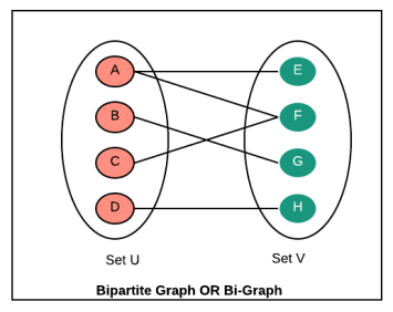
먼저 무비렌즈 데이터셋을 그래프 자료구조로 바꿔보자. PinSAGE, MultiSAGE 알고리즘은 기본적으로 bi-partite 형태의 그래프 자료구조를 사용한다는 전제로 진행된다. 이는 Metapath(Movie - User - Movie)를 통해 영화 간의 연결 정보를 유저라는 중간 매개체로 담아내고, 결과적으로는 영화 자체를 임베딩한다.

 

users = []
with open(os.path.join(directory, 'users.dat'), encoding='latin1') as f:
    for l in f:
        id_, gender, age, occupation, zip_ = l.strip().split('::')
        users.append({
            'user_id': int(id_),
            'gender': gender,
            'age': age,
            'occupation': occupation,
            'zip': zip_,
        })
users = pd.DataFrame(users).astype('category')

movies = []
with open(os.path.join(directory, 'movies.dat'), encoding='latin1') as f:
    for l in f:
        id_, title, genres = l.strip().split('::')
        genres_set = set(genres.split('|'))

        # extract year
        assert re.match(r'.*\([0-9]{4}\)$', title)
        year = title[-5:-1]
        title = title[:-6].strip()

        data = {'movie_id': int(id_), 'title': title, 'year': year}
        for g in genres_set:
            data[g] = True
        movies.append(data)
movies = pd.DataFrame(movies).astype({'year': 'category'})

ratings = []
with open(os.path.join(directory, 'ratings.dat'), encoding='latin1') as f:
    for l in f:
        user_id, movie_id, rating, timestamp = [int(_) for _ in l.split('::')]
        ratings.append({
            'user_id': user_id,
            'movie_id': movie_id,
            'rating': rating,
            'timestamp': timestamp,
        })
ratings = pd.DataFrame(ratings)

distinct_users_in_ratings = ratings['user_id'].unique()
distinct_movies_in_ratings = ratings['movie_id'].unique()
users = users[users['user_id'].isin(distinct_users_in_ratings)]
movies = movies[movies['movie_id'].isin(distinct_movies_in_ratings)]

genre_columns = movies.columns.drop(['movie_id', 'title', 'year'])
movies[genre_columns] = movies[genre_columns].fillna(False).astype('bool')
movies_categorical = movies.drop('title', axis=1)

graph_builder = PandasGraphBuilder()
graph_builder.add_entities(users, 'user_id', 'user')
graph_builder.add_entities(movies_categorical, 'movie_id', 'movie')
graph_builder.add_binary_relations(ratings, 'user_id', 'movie_id', 'watched')
graph_builder.add_binary_relations(ratings, 'movie_id', 'user_id', 'watched-by')
g = graph_builder.build()

g.nodes['movie'].data['year'] = torch.LongTensor(movies['year'].cat.codes.values)
g.nodes['movie'].data['genre'] = torch.FloatTensor(movies[genre_columns].values)
g.edges['watched'].data['rating'] = torch.LongTensor(ratings['rating'].values)
g.edges['watched'].data['timestamp'] = torch.LongTensor(ratings['timestamp'].values)
g.edges['watched-by'].data['rating'] = torch.LongTensor(ratings['rating'].values)
g.edges['watched-by'].data['timestamp'] = torch.LongTensor(ratings['timestamp'].values)

 

이제 Metapath(Movie - User - Movie) 정보를 가지고 있는 그래프 객체 g가 생성되었고, 여기에 torch에서 바로 학습할 수 있는 형태의 Feature Vector들도 만들어준다.

 

---

 

PinSAGE Sampling for pair Similarity

 

GraphSAGE 알고리즘은 Convolution을 수행할 수 있는 형태로 인접 노드를 샘플링해야 한다. 논문의 샘플링 방식인 PinSAGE는 이웃을 완전한 uniform random sampling으로 추출하는 것이 아닌, PPR에 기반한 Random Walks로 추출한다. 즉, 하나의 노드를 샘플링 할 때는 Page Rank Edge Score를 기준으로 링크가 강한 연결관계를 위주로 랜덤 샘플링을 진행한다. 이러한 PinSAGE 샘플링은 dgl 라이브러리에서 손쉽게 사용할 수 있다. 아래 코드에서 self.samplers 부분이 바로 PinSAGE 샘플링 객체 선언 부분이다.

 

class NeighborSampler(object):
    def __init__(self, g, user_type, item_type, random_walk_length, random_walk_restart_prob,
                 num_random_walks, num_neighbors, num_layers):
        self.g = g
        self.user_type = user_type
        self.item_type = item_type
        self.user_to_item_etype = list(g.metagraph()[user_type][item_type])[0]
        self.item_to_user_etype = list(g.metagraph()[item_type][user_type])[0]
        self.samplers = [
            dgl.sampling.PinSAGESampler(g, item_type, user_type, random_walk_length,
                                        random_walk_restart_prob, num_random_walks, num_neighbors)
            for _ in range(num_layers)]

    def sample_blocks(self, seeds, heads=None, tails=None, neg_tails=None):
        blocks = []
        for sampler in self.samplers:
            frontier = sampler(seeds)
            if heads is not None:
                eids = frontier.edge_ids(torch.cat([heads, heads]), torch.cat([tails, neg_tails]), return_uv=True)[2]
                if len(eids) > 0:
                    old_frontier = frontier
                    frontier = dgl.remove_edges(frontier, eids)
            block = compact_and_copy(frontier, seeds)
            seeds = block.srcdata[dgl.NID]
            blocks.insert(0, block) 
        return blocks

    def sample_from_item_pairs(self, heads, tails, neg_tails):
        pos_graph = dgl.graph(
            (heads, tails),
            num_nodes=self.g.number_of_nodes(self.item_type))
        neg_graph = dgl.graph(
            (heads, neg_tails),
            num_nodes=self.g.number_of_nodes(self.item_type))
        pos_graph, neg_graph = dgl.compact_graphs(
            [pos_graph, neg_graph])
        seeds = pos_graph.ndata[dgl.NID]
        blocks = self.sample_blocks(seeds, heads, tails, neg_tails)
        return pos_graph, neg_graph, blocks

 

PinSAGESampler 클래스로 샘플링을 하려면, 샘플링의 대상이 되는 seed id들을 입력해주어야 한다. 그래서 샘플링에 필요한 Positive-Nodes와 Negative-Nodes에 해당하는 seed ids를 우선적으로 정의한 뒤에 샘플링을 진행한다. Positive 노드는 Target 노드로부터 Random Walk를 수행하여 n-depth 시뮬레이션 내에 포함되는 노드들을 의미하며, Negative 노드는 그래프 연결관계와 상관 없이 완전하게 랜덤으로 샘플링된 노드들을 의미한다. 데이터셋이 커지면 커질수록 Positive-Negative를 구분하는 것이 확률적으로 정확해질 것이다. seed ids를 출력하는 코드는 아래와 같다. heads가 시작 노드, tails가 positive nodes, neg_tails가 negative nodes를 의미한다.

 

heads = torch.randint(0, self.g.number_of_nodes(self.item_type), (self.batch_size,))
result = dgl.sampling.random_walk(
    self.g,
    heads,
    metapath=[self.item_to_user_etype, self.user_to_item_etype])
tails = result[0][:, 2]
neg_tails = torch.randint(0, self.g.number_of_nodes(self.item_type), (self.batch_size,))
mask = (tails != -1)
yield heads[mask], tails[mask], neg_tails[mask]

 

모델을 학습하는 과정에서는 Positive-Nodes와 Negative-Nodes를 각각 모델에 적용하여 Low-rank positives 랭킹 학습을 수행하기 때문에, 샘플링과 동시에 학습 과정에서 분리할 positive sub-graph, negative sub-graph도 각각 정의해둔다. sample_from_item_pairs 함수가 그 역할을 수행한다.

 

---

 

Graph Convolutional Layers

 

GNN의 레이어 구조를 torch 코드로 간단하게 알아보자. dgl의 block 구조를 사용해야 하는 부분을 제외하면, 레이어를 디자인하는 과정은 어렵지 않다.

 

먼저 PinSAGE 샘플링을 사용한 GraphSAGE 모델의 클래스를 코드로 정의해보자.

 

Model Structure

class PinSAGEModel(nn.Module):
    def __init__(self, full_graph, ntype, hidden_dims, n_layers):
        super().__init__()
        self.proj = layers.LinearProjector(full_graph, ntype, hidden_dims)
        self.sage = layers.SAGENet(hidden_dims, n_layers)
        self.scorer = layers.ItemToItemScorer(full_graph, ntype)

    def forward(self, pos_graph, neg_graph, blocks):
        h_item = self.get_representation(blocks)
        pos_score = self.scorer(pos_graph, h_item)
        neg_score = self.scorer(neg_graph, h_item)
        return (neg_score - pos_score + 1).clamp(min=0)

    def get_representation(self, blocks):
        h_item = self.proj(blocks[0].srcdata)
        h_item_dst = self.proj(blocks[-1].dstdata)
        return h_item_dst + self.sage(blocks, h_item)
        
        
class ItemToItemScorer(nn.Module):
    def __init__(self, full_graph, ntype):
        super().__init__()
        n_nodes = full_graph.number_of_nodes(ntype)
        self.bias = nn.Parameter(torch.zeros(n_nodes))

    def _add_bias(self, edges):
        bias_src = self.bias[edges.src[dgl.NID]]
        bias_dst = self.bias[edges.dst[dgl.NID]]
        return {'s': edges.data['s'] + bias_src + bias_dst}

    def forward(self, item_item_graph, h):
        with item_item_graph.local_scope():
            item_item_graph.ndata['h'] = h
            item_item_graph.apply_edges(fn.u_dot_v('h', 'h', 's'))
            item_item_graph.apply_edges(self._add_bias)
            pair_score = item_item_graph.edata['s']
        return pair_score

논문에서 Projection Layer에 해당하는 부분들을 self.proj로 정의한다. 이 레이어는 노드의 input feature들을 projection 하는 레이어들의 모듈로 구성이 되어있다. forward 함수는 Positive Nodes, Negative Nodes의 sub-graph를 인자로 받으며, 또한 이 노드들의 정보를 모두 포함하고 있는 block라는 dgl 패키지의 자료구조를 입력받는다. pos_graph, neg_graph는 일종의 포인터이고, 실제 자료는 blocks 라고 생각하면 된다.

 

그 결과 각각 임베딩 벡터를 만들어내고, Scorer 객체를 통해 score를 계산하여 low-rank positive를 계산한다.

 

 

Projection Layer

def _init_input_modules(g, ntype, hidden_dims):
    module_dict = nn.ModuleDict()
    for column, data in g.nodes[ntype].data.items():
        if column == dgl.NID:
            continue
        if data.dtype == torch.float32:
            assert data.ndim == 2
            m = nn.Linear(data.shape[1], hidden_dims)
            nn.init.xavier_uniform_(m.weight)
            nn.init.constant_(m.bias, 0)
            module_dict[column] = m
        elif data.dtype == torch.int64:
            assert data.ndim == 1
            m = nn.Embedding(data.max() + 2, hidden_dims, padding_idx=-1)
            nn.init.xavier_uniform_(m.weight)
            module_dict[column] = m
    return module_dict


class LinearProjector(nn.Module):
    def __init__(self, full_graph, ntype, hidden_dims):
        super().__init__()
        self.ntype = ntype
        self.inputs = _init_input_modules(full_graph, ntype, hidden_dims)

    def forward(self, ndata):
        projections = []
        for feature, data in ndata.items():
            if feature == dgl.NID or feature.endswith('__len'):
                continue
            module = self.inputs[feature]
            result = module(data)
            projections.append(result)
        return torch.stack(projections, 1).sum(1)

위 코드는 간단하게 GCN 모델의 Projection Layer를 구현한 것이다. Projection Layer는 노드 피처들이 모두 같은 shape의 output으로 나오게 하여, aggregate 할 수 있는 형태로 만들어야 한다. 그리고 이 결과를 코드에서는 torch.stack() 으로 aggregate 하였다.

 

 

Convolutional Structure

class SAGENet(nn.Module):
    def __init__(self, hidden_dims, n_layers):
        super().__init__()
        self.convs = nn.ModuleList()
        for _ in range(n_layers):
            self.convs.append(WeightedSAGEConv(hidden_dims, hidden_dims, hidden_dims))

    def forward(self, blocks, h):
        for layer, block in zip(self.convs, blocks):
            h_dst = h[:block.number_of_nodes('DST/' + block.ntypes[0])]
            h = layer(block, (h, h_dst), block.edata['weights'])
        return h

NeighborSampler 클래스의 sample_blocks로 샘플링을 실행하면 blocks에 n-length의 리스트가 반환된다. blocks[0]은 Convolution 할 Sub-graph에서 "2-depth neighbor nodes to 1-depth neighbor nodes"에 관한 정보를 가지고 있고, blocks[1] 혹은 blocks[-1]은 "1-depth neighbor to target nodes"에 관한 정보를 가지고 있다. 이 계층적 구조에 맞게 Convolution Layer를 n번 수행하는 반복 레이어 구조를 정의한 것이 SAGENet 클래스이다.

 

 

GraphSAGE Layer

class WeightedSAGEConv(nn.Module):
    def __init__(self, input_dims, hidden_dims, output_dims, act=F.relu):
        super().__init__()
        self.act = act
        self.Q = nn.Linear(input_dims, hidden_dims)
        self.W = nn.Linear(input_dims + hidden_dims, output_dims)
        self.reset_parameters()
        self.dropout = nn.Dropout(0.5)

    def reset_parameters(self):
        gain = nn.init.calculate_gain('relu')
        nn.init.xavier_uniform_(self.Q.weight, gain=gain)
        nn.init.xavier_uniform_(self.W.weight, gain=gain)
        nn.init.constant_(self.Q.bias, 0)
        nn.init.constant_(self.W.bias, 0)

    def forward(self, block, h, weights):
        h_src, h_dst = h
        with block.local_scope():
            block.srcdata['nft'] = self.act(self.Q(self.dropout(h_src)))
            block.edata['w'] = weights.float()
            block.update_all(fn.u_mul_e('nft', 'w', 'm'), fn.sum('m', 'nft'))
            block.update_all(fn.copy_e('w', 'm'), fn.sum('m', 'ws'))
            n = block.dstdata['nft']
            ws = block.dstdata['ws'].unsqueeze(1).clamp(min=1)
            z = self.act(self.W(self.dropout(torch.cat([n / ws, h_dst], 1))))
            z_norm = z.norm(2, 1, keepdim=True)
            z_norm = torch.where(z_norm == 0, torch.tensor(1.).to(z_norm), z_norm)
            z = z / z_norm
            return z

대부분의 계산이 이루어지는 핵심 레이어라고 할수 있는 것이 WeightedSAGEConv 클래스이다. Projection 된 입력값을 FC Layer에 한번 더 통과시켜 준 뒤, Message Passing을 통하여 논문에 있는 내용대로 Convolution Task를 수행한다. 이는 PinSAGE Sampling에서 계산된 PPR score를 Node feature와 행렬곱 해주는 과정을 포함하며, 연산 이후에는 다시 한 번 FC Layer를 거쳐 Normalize까지 씌워준다.

 

---

 

Result & Visualize

 

모델을 학습한 뒤, Movie 단위로 임베딩 벡터를 생성할 수 있을 것이다. 이제 임베딩이 잘 됐는지 확인해보자.

 

PinSAGE는 기본적으로 노드간의 컨텍스트 기반 유사성을 매개로 학습하는 것이기 때문에, MovieLens 데이터셋에 적용하면 영화 벡터간의 유사도를 구하는 것에 대단히 용이할 것이다.

 

scipy의 KDTree 알고리즘으로 특정 영화 벡터와 유사한 다른 영화 벡터들을 찾아보자.

 

import re

import pandas as pd
import numpy as np
from scipy import spatial


movies = []
with open('./dataset/movielens/movies.dat', encoding='latin1') as f:
    for l in f:
        id_, title, genres = l.strip().split('::')
        genres_set = set(genres.split('|'))

        # extract year
        assert re.match(r'.*\([0-9]{4}\)$', title)
        year = title[-5:-1]
        title = title[:-6].strip()

        data = {'movie_id': int(id_), 'title': title, 'year': year}
        for g in genres_set:
            data[g] = True
        movies.append(data)
movies = pd.DataFrame(movies).astype({'year': 'category'})

ratings = []
with open('./dataset/movielens/ratings.dat', encoding='latin1') as f:
    for l in f:
        user_id, movie_id, rating, timestamp = [int(_) for _ in l.split('::')]
        ratings.append({
            'user_id': user_id,
            'movie_id': movie_id,
            'rating': rating,
            'timestamp': timestamp,
            })
ratings = pd.DataFrame(ratings)

distinct_users_in_ratings = ratings['user_id'].unique()
distinct_movies_in_ratings = ratings['movie_id'].unique()
movies = movies[movies['movie_id'].isin(distinct_movies_in_ratings)]

genre_columns = movies.columns.drop(['movie_id', 'title', 'year'])
movies[genre_columns] = movies[genre_columns].fillna(False).astype('bool')
movies_categorical = movies.drop('title', axis=1)

entities = movies['movie_id'].astype('category')
entities = entities.cat.reorder_categories(movies['movie_id'].values)

index_id_to_movie_id = {}
movie_id_to_index_id = {}
for idx, movie_id in enumerate(entities):
    index_id_to_movie_id[idx] = movie_id
    movie_id_to_index_id[movie_id] = idx

saved_npz = np.load('./pinsage/' + 'h_items.npz')
h_item = saved_npz['movie_vectors']
tree = spatial.KDTree(h_item.tolist())
tree.query(h_item[movie_id_to_index_id[1]].tolist(), 10)

index_ids = tree.query(h_item[movie_id_to_index_id[1]].tolist(), 10)[1]
movie_ids = [index_id_to_movie_id[idx] for idx in index_ids]
for mid in movie_ids:
    print(movies[movies['movie_id']==mid]['title'].values)

그럼, [Toy Story]와 유사한 영화가 아래처럼 검색된다.

['Toy Story']
['Balto']
['Gumby: The Movie']
['Land Before Time III: The Time of the Great Giving']
['Goofy Movie, A']
['Aladdin and the King of Thieves']
["Bug's Life, A"]
['Rugrats Movie, The']
['Big Green, The']
['Toy Story 2']

 

이렇게 PinSAGE 알고리즘을 간단하게 pytorch로 구현해보았다. 여기까지는 공개되어있는 예제를 크게 바꾸지 않았기 때문에, 쉽게 정보를 얻을 수 있을 것이다. 하지만 MultiSAGE를 구현할 때는 dgl 패키지도 조금 수정해야 하고, Attention Layer와 Message Passing을 직접 구현해야 한다. 다음 포스팅에서는 이 내용을 알아보겠다. GAT 개념을 도입하여 영화의 Genre를 Context로, Indexed Attention을 계산할 수 있는 MultiSAGE 알고리즘을 구현한 내용을 포함할 것이다.